Introduction
To illustrate the functionality of the dar package, this study will use the data set from (Noguera-Julian, M., et al. 2016). The authors of this study found that men who have sex with men (MSM) predominantly belonged to the Prevotella-rich enterotype whereas most non-MSM subjects were enriched in Bacteroides, independently of HIV-1 status. This result highlights the potential impact of sexual orientation on the gut microbiome and emphasizes the importance of controlling for such variables in microbiome research. Using the dar package, we will conduct a differential abundance analysis to further explore this finding and uncover potential microbial biomarkers associated with this specific population.
Recipe Initialization
To begin the analysis process with the dar package, the
first step is to initialize a Recipe object, which is an S4 class. This
recipe object serves as a blueprint for the data preparation steps
required for the differential abundance analysis. The initialization of
the recipe object is done through the function recipe(),
which takes as inputs a phyloseq or
TreeSummarizedExperiment (TSE) object, the name of the
categorical variable of interest and the taxonomic level at which the
differential abundance analyses are to be performed. As previously
mentioned, we will use the data set from (Noguera-Julian, M., et
al. 2016) and the variable of interest “RiskGroup2” containing the
categories: men who have sex with men (msm), non-MSM (hts) and people
who inject drugs (pwid) and we will perform the analysis at the species
level.
# Recipe Initialization
rec <- recipe(metaHIV_phy, var_info = "RiskGroup2", tax_info = "Species")
rec
#> ── DAR Recipe ──────────────────────────────────────────────────────────────────
#> Inputs:
#>
#>      ℹ phyloseq object with 451 taxa and 156 samples
#>      ℹ variable of interes RiskGroup2 (class: character, levels: hts, msm, pwid)
#>      ℹ taxonomic level Species
Recipe QC and Preprocessing Steps Definition
Once the recipe object has been initialized, the next step is to
populate it with steps. Steps are the methods that will be applied to
the data stored in the recipe. There are two types of steps:
preprocessing (prepro) and differential abundance (da) steps. Initially,
we will focus on the prepro steps which are used to modify the data
loaded into the recipe, which will then be used for the da steps. The
dar package includes 3 main preprocessing functionalities:
step_subset_taxa, which is used for subsetting columns and
values in the taxon table connected to the phyloseq object,
step_filter_taxa, which is used to filter the OTUs, and
step_rarefaction, which is used to resample the OTU table
to ensure that all samples have the same library size. These
functionalities allow for a high level of flexibility and customization
in the data preparation process before performing the differential
abundance analysis.
The dar package provides convenient wrappers for the step_filter_taxa function, designed to filter Operational Taxonomic Units (OTUs) based on specific criteria: prevalence, variance, abundance, and rarity.
-
step_filter_by_prevalence: Filters OTUs according to the number of samples in which the OTU appears. -
step_filter_by_variance: Filters OTUs based on the variance of the OTU’s presence across samples. -
step_filter_by_abundance: Filters OTUs according to the OTU’s abundance across samples. -
step_filter_by_rarity: Filters OTUs based on the rarity of the OTU across samples.
In addition to the preprocessing steps, the dar package also
incorporates the function phy_qc which returns a table with a set of
metrics that allow for informed decisions to be made about the data
preprocessing that will be done. In our case, we decided to use the
step_subset_taxa function to retain only those observations
annotated within the realm of Bacteria and Archaea. We also used the
step_filter_by_prevalence function to retain only those
OTUs with at least 1% of the samples with values greater than 0. This
approach ensured that we were working with a high-quality, informative
subset of the data, which improved the overall accuracy and reliability
of the differential abundance analysis.
# Summary Stats by levels
phy_qc(rec)
#> # A tibble: 4 × 12
#>   var_levels     n n_zero pct_zero pct_all_zero pct_singletons pct_doubletons
#>   <chr>      <int>  <int>    <dbl>        <dbl>          <dbl>          <dbl>
#> 1 all        70356  57632     81.9          0             20.6           8.87
#> 2 hts        18491  15108     81.7         24.2           22.8           8.43
#> 3 msm        45100  37019     82.1         16.0           20.2           9.53
#> 4 pwid        6765   5505     81.4         41.2           16.6           9.31
#> # ℹ 5 more variables: n_samples <int>, lib_size_min <dbl>, lib_size_max <dbl>,
#> #   count_mean <dbl>, count_max <dbl>

# Adding prepro steps
rec <-
  rec |>
  step_subset_taxa(tax_level = "Kingdom", taxa = c("Bacteria", "Archaea")) |>
  step_filter_by_prevalence()

rec
#> ── DAR Recipe ──────────────────────────────────────────────────────────────────
#> Inputs:
#>
#>      ℹ phyloseq object with 451 taxa and 156 samples
#>      ℹ variable of interes RiskGroup2 (class: character, levels: hts, msm, pwid)
#>      ℹ taxonomic level Species
#>
#> Preporcessing steps:
#>
#>      ◉ step_subset_taxa() id = subset_taxa__Bridie
#>      ◉ step_filter_by_prevalence() id = filter_by_prevalence__Gujiya
#>
#> DA steps:
Define Differential Analysis (DA) steps
Once data is preprocessed and cleaned, the next step is to add the da
steps. The dar package incorporates multiple methods to analyze the
data, including: ALDEx2, ANCOM-BC,
corncob, DESeq2, Lefse,
MAaslin3, and Wilcox. These methods provide a
range of options for uncovering potential microbial biomarkers
associated with the variable of interest. To ensure consistency across
methods, we decided not to use default parameters, but to set the
min_prevalence parameter to 0 for MAaslin2.
This approach ensured that the analysis was consistent across all
methods and that the results were interpretable.
# DA steps definition
rec <-
  rec |>
  step_wilcox() |>
  # step_ancom() |>
  step_aldex() |>
  step_deseq() |>
  step_corncob(filter_discriminant = FALSE) |>
  step_maaslin(min_prevalence = 0) |>
  step_lefse()

rec
#> ── DAR Recipe ──────────────────────────────────────────────────────────────────
#> Inputs:
#>
#>      ℹ phyloseq object with 451 taxa and 156 samples
#>      ℹ variable of interes RiskGroup2 (class: character, levels: hts, msm, pwid)
#>      ℹ taxonomic level Species
#>
#> Preporcessing steps:
#>
#>      ◉ step_subset_taxa() id = subset_taxa__Bridie
#>      ◉ step_filter_by_prevalence() id = filter_by_prevalence__Gujiya
#>
#> DA steps:
#>
#>      ◉ step_wilcox() id = wilcox__Paper_wrapped_cake
#>      ◉ step_aldex() id = aldex__Klobasnek
#>      ◉ step_deseq() id = deseq__Kroštule
#>      ◉ step_corncob() id = corncob__Muskazine
#>      ◉ step_maaslin() id = maaslin__Milk_cream_strudel
#>      ◉ step_lefse() id = lefse__Poffertjes
Prep recipe
Once the recipe has been defined, the next step is to
execute all the steps defined in the recipe. This is done
through the function prep(). Internally, it first executes
the preprocessing steps, which modify the phyloseq object
stored in the recipe. Then, using the modified
phyloseq, it executes each of the defined differential
abundance methods. To speed up the execution time, the
prep() function includes the option to run in parallel. The
resulting object has class PrepRecipe and when printed in
the terminal, it displays the number of taxa detected as significant in
each of the methods and also the total number of taxa shared across all
methods. This allows for a provisional overview of the results and a
comparison between methods.
# Execute in parallel
da_results <- prep(rec, parallel = TRUE)
#> Warning in lefser::lefser(se, classCol = var, kruskal.threshold = 1,
#> wilcox.threshold = 1, : Variables in the input are collinear. Try only with the
#> terminal nodes using `get_terminal_nodes` function
#> Warning in lefser::lefser(se, classCol = var, kruskal.threshold = 1,
#> wilcox.threshold = 1, : Variables in the input are collinear. Try only with the
#> terminal nodes using `get_terminal_nodes` function
#> Warning in lefser::lefser(se, classCol = var, kruskal.threshold = 1,
#> wilcox.threshold = 1, : Variables in the input are collinear. Try only with the
#> terminal nodes using `get_terminal_nodes` function

da_results
#> ── DAR Results ─────────────────────────────────────────────────────────────────
#> Inputs:
#>
#>      ℹ phyloseq object with 355 taxa and 156 samples
#>      ℹ variable of interes RiskGroup2 (class: character, levels: hts, msm, pwid)
#>      ℹ taxonomic level Species
#>
#> Results:
#>
#>      ✔ wilcox__Paper_wrapped_cake diff_taxa = 183
#>      ✔ aldex__Klobasnek diff_taxa = 93
#>      ✔ deseq__Kroštule diff_taxa = 174
#>      ✔ corncob__Muskazine diff_taxa = 135
#>      ✔ maaslin__Milk_cream_strudel diff_taxa = 58
#>      ✔ lefse__Poffertjes diff_taxa = 117
#>
#>      ℹ 19 taxa are present in all tested methods
Default results extraction
At this point, we could extract the taxa shared across all methods
using the function bake() to define a default consensus
strategy and then cool() to extract the results.
# Default DA taxa results
results <-
  bake(da_results) |>
  cool()

results
#> # A tibble: 19 × 2
#>    taxa_id taxa
#>    <chr>   <chr>
#>  1 Otu_35  Collinsella_aerofaciens
#>  2 Otu_47  Bacteroides_cellulosilyticus
#>  3 Otu_63  Bacteroides_plebeius
#>  4 Otu_69  Bacteroides_sp_CAG_530
#>  5 Otu_78  Bacteroides_uniformis
#>  6 Otu_82  Barnesiella_intestinihominis
#>  7 Otu_96  Prevotella_copri
#>  8 Otu_102 Prevotella_sp_AM42_24
#>  9 Otu_115 Alistipes_finegoldii
#> 10 Otu_119 Alistipes_putredinis
#> 11 Otu_130 Parabacteroides_sp_CAG_409
#> 12 Otu_234 Eubacterium_ramulus
#> 13 Otu_255 Ruminococcus_torques
#> 14 Otu_258 Coprococcus_catus
#> 15 Otu_259 Coprococcus_comes
#> 16 Otu_261 Dorea_formicigenerans
#> 17 Otu_262 Dorea_longicatena
#> 18 Otu_332 Catenibacterium_mitsuokai
#> 19 Otu_365 Mitsuokella_jalaludinii
However, dar allows for complex consensus strategies
based on the obtained results. To that end, the user has access to
different functions to graphically represent different types of
information. This feature allows for a more in-depth analysis of the
results and a better understanding of the underlying patterns in the
data.
Exploration for consensus strategie definition
For example, intersection_plt() gives an overview of the
overlaps between methods by creating an upSet plot. In our case, this
function has shown that 24 taxa are shared across all the methods
used.
# Intersection plot
intersection_plt(da_results, ordered_by = "degree", font_size = 1)
#> Warning: `aes_string()` was deprecated in ggplot2 3.0.0.
#> ℹ Please use tidy evaluation idioms with `aes()`.
#> ℹ See also `vignette("ggplot2-in-packages")` for more information.
#> ℹ The deprecated feature was likely used in the UpSetR package.
#>   Please report the issue to the authors.
#> This warning is displayed once per session.
#> Call `lifecycle::last_lifecycle_warnings()` to see where this warning was
#> generated.
#> Warning: Using `size` aesthetic for lines was deprecated in ggplot2 3.4.0.
#> ℹ Please use `linewidth` instead.
#> ℹ The deprecated feature was likely used in the UpSetR package.
#>   Please report the issue to the authors.
#> This warning is displayed once per session.
#> Call `lifecycle::last_lifecycle_warnings()` to see where this warning was
#> generated.
#> Warning: The `size` argument of `element_line()` is deprecated as of ggplot2 3.4.0.
#> ℹ Please use the `linewidth` argument instead.
#> ℹ The deprecated feature was likely used in the UpSetR package.
#>   Please report the issue to the authors.
#> This warning is displayed once per session.
#> Call `lifecycle::last_lifecycle_warnings()` to see where this warning was
#> generated.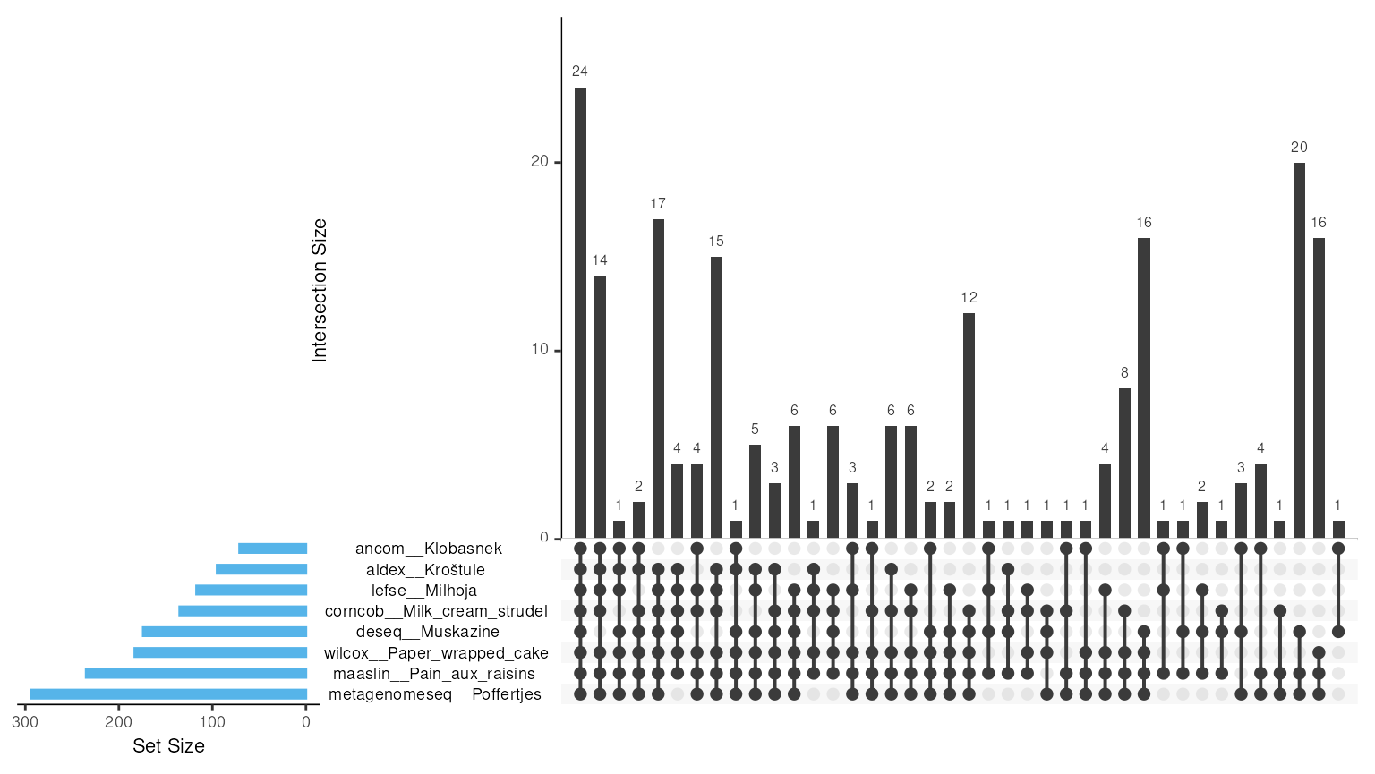
In addition to the intersection_plt() function, dar also
has the function exclusion_plt() which provides information
about the number of OTUs shared between methods. This function allows to
identify the OTUs that are specific to each method and also the ones
that are not shared among any method.
# Exclusion plot
exclusion_plt(da_results)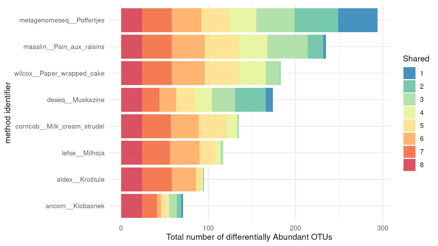
Besides to the previously mentioned functions, dar also includes the
function corr_heatmap(), which allows for visualization of
the overlap of significant OTUs between tested methods. This function
can provide similar information to the previous plots, but in some cases
it may be easier to interpret. comprehensive view of the results.
# Correlation heatmap
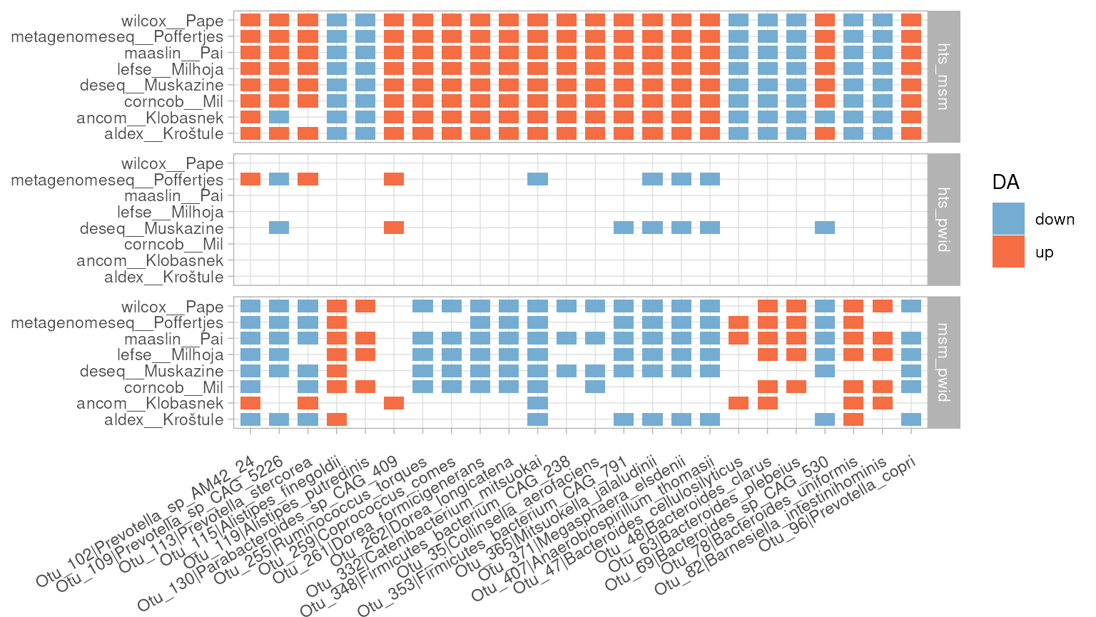
corr_heatmap(da_results, font_size = 10) Finally, dar also includes the function
mutual_plt(), which plots the number of differential
abundant features mutually found by a defined number of methods, colored
by the differential abundance direction and separated by comparison. The
resulting graph allows us to see that the features detected correspond
mainly to the comparisons between hts vs msm and msm vs pwid.
Additionally, the graph also allows us to observe the direction of the
effect, whether a specific OTU is enriched or depleted for each
comparison.
# Mutual plot
mutual_plt(
  da_results,
  count_cutoff = length(steps_ids(da_results, type = "da")),
  top_n = 24
)
Define a consesus strategy using bake
After visually inspecting the results from running all the
differential analysis methods on our data, we have the necessary
information to define a consensus strategy that fits our dataset. In our
case, we will retain all the methods. However if one or more methods are
not desired, the bake() function includes the
exclude parameter, which allows to exclude specific
methods.
Additionally, the bake() function allows to further
refine the consensus strategy through its parameters, such as
count_cutoff, which indicates the minimum number of methods
in which an OTU must be present, and weights, a named vector with the
ponderation value for each method. However, for simplicity, these
parameters are not used in this example.
# Define consensus strategy
da_results <- bake(da_results)
da_results
#> ── DAR Results ─────────────────────────────────────────────────────────────────
#> Inputs:
#>
#>      ℹ phyloseq object with 355 taxa and 156 samples
#>      ℹ variable of interes RiskGroup2 (class: character, levels: hts, msm, pwid)
#>      ℹ taxonomic level Species
#>
#> Results:
#>
#>      ✔ wilcox__Paper_wrapped_cake diff_taxa = 183
#>      ✔ aldex__Klobasnek diff_taxa = 93
#>      ✔ deseq__Kroštule diff_taxa = 174
#>      ✔ corncob__Muskazine diff_taxa = 135
#>      ✔ maaslin__Milk_cream_strudel diff_taxa = 58
#>      ✔ lefse__Poffertjes diff_taxa = 117
#>
#>      ℹ 19 taxa are present in all tested methods
#>
#> Bakes:
#>
#>      ◉ 1 -> count_cutoff: NULL, weights: NULL, exclude: NULL, id: bake__Knish
Extract results
To conclude, we can extract the final results using the
cool() function. This function takes a
PrepRecipe object and the ID of the bake to be used as
input (by default it is 1, but if you have multiple consensus
strategies, you can change it to extract the desired results).
# Extract results for bake id 1
f_results <- cool(da_results, bake = 1)

f_results
#> # A tibble: 19 × 2
#>    taxa_id taxa
#>    <chr>   <chr>
#>  1 Otu_35  Collinsella_aerofaciens
#>  2 Otu_47  Bacteroides_cellulosilyticus
#>  3 Otu_63  Bacteroides_plebeius
#>  4 Otu_69  Bacteroides_sp_CAG_530
#>  5 Otu_78  Bacteroides_uniformis
#>  6 Otu_82  Barnesiella_intestinihominis
#>  7 Otu_96  Prevotella_copri
#>  8 Otu_102 Prevotella_sp_AM42_24
#>  9 Otu_115 Alistipes_finegoldii
#> 10 Otu_119 Alistipes_putredinis
#> 11 Otu_130 Parabacteroides_sp_CAG_409
#> 12 Otu_234 Eubacterium_ramulus
#> 13 Otu_255 Ruminococcus_torques
#> 14 Otu_258 Coprococcus_catus
#> 15 Otu_259 Coprococcus_comes
#> 16 Otu_261 Dorea_formicigenerans
#> 17 Otu_262 Dorea_longicatena
#> 18 Otu_332 Catenibacterium_mitsuokai
#> 19 Otu_365 Mitsuokella_jalaludinii
To further visualize the results, the abundance_plt()
function can be utilized to visualize the differences in abundance of
the differential abundant taxa.
# Ids for Bacteroide and Provotella species
ids <-
  f_results |>
  dplyr::filter(stringr::str_detect(taxa, "Bacteroi.*|Prevote.*")) |>
  dplyr::pull(taxa_id)

# Abundance plot as boxplot
abundance_plt(da_results, taxa_ids = ids, type = "boxplot") 
# Abundance plot as heatmap
abundance_plt(da_results, type = "heatmap", transform = "compositional")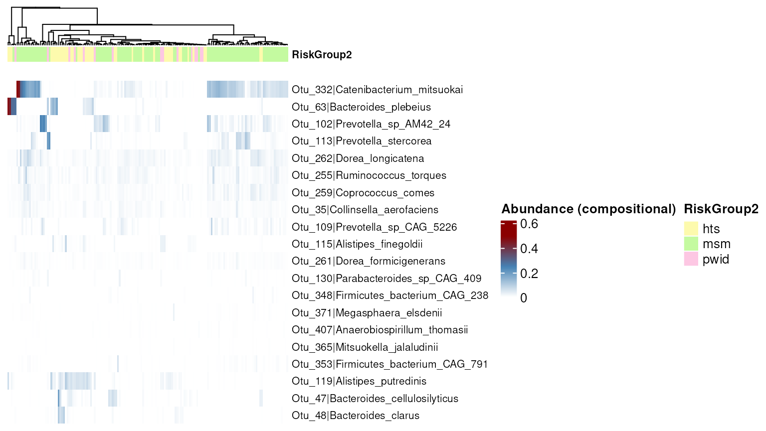
Session Info
devtools::session_info()
#> ─ Session info ───────────────────────────────────────────────────────────────
#> setting value
#> version R version 4.5.2 (2025-10-31)
#> os Ubuntu 24.04.3 LTS
#> system x86_64, linux-gnu
#> ui X11
#> language en
#> collate en_US.UTF-8
#> ctype en_US.UTF-8
#> tz UTC
#> date 2026-04-29
#> pandoc 3.8.2.1 @ /usr/bin/ (via rmarkdown)
#> quarto 1.7.32 @ /usr/local/bin/quarto
#>
#> ─ Packages ───────────────────────────────────────────────────────────────────
#> package * version date (UTC) lib source
#> abind 1.4-8 2024-09-12 [1] RSPM (R 4.5.0)
#> ade4 1.7-24 2026-03-21 [1] RSPM (R 4.5.0)
#> ALDEx2 1.42.0 2025-10-29 [1] Bioconductor 3.22 (R 4.5.2)
#> ape 5.8-1 2024-12-16 [1] RSPM (R 4.5.0)
#> apeglm 1.32.0 2025-10-29 [1] Bioconductor 3.22 (R 4.5.2)
#> aplot 0.2.9 2025-09-12 [1] RSPM (R 4.5.0)
#> ashr 2.2-63 2023-08-21 [1] RSPM (R 4.5.0)
#> assertthat 0.2.1 2019-03-21 [1] RSPM (R 4.5.0)
#> backports 1.5.1 2026-04-03 [1] RSPM (R 4.5.0)
#> bbmle 1.0.25.1 2023-12-09 [1] RSPM (R 4.5.0)
#> bdsmatrix 1.3-7 2024-03-02 [1] RSPM (R 4.5.0)
#> beachmat 2.26.0 2025-10-29 [1] Bioconductor 3.22 (R 4.5.2)
#> beeswarm 0.4.0 2021-06-01 [1] RSPM (R 4.5.0)
#> Biobase 2.70.0 2025-10-29 [1] Bioconductor 3.22 (R 4.5.2)
#> BiocBaseUtils 1.12.0 2025-10-29 [1] Bioconductor 3.22 (R 4.5.2)
#> BiocGenerics 0.56.0 2025-10-29 [1] Bioconductor 3.22 (R 4.5.2)
#> BiocNeighbors 2.4.0 2025-10-29 [1] Bioconductor 3.22 (R 4.5.2)
#> BiocParallel 1.44.0 2025-10-29 [1] Bioconductor 3.22 (R 4.5.2)
#> BiocSingular 1.26.1 2025-11-17 [1] Bioconductor 3.22 (R 4.5.2)
#> biomformat 1.38.3 2026-03-16 [1] Bioconductor 3.22 (R 4.5.2)
#> Biostrings 2.78.0 2025-10-29 [1] Bioconductor 3.22 (R 4.5.2)
#> bitops 1.0-9 2024-10-03 [1] RSPM (R 4.5.0)
#> bluster 1.20.0 2025-10-29 [1] Bioconductor 3.22 (R 4.5.2)
#> brio 1.1.5 2024-04-24 [2] RSPM (R 4.5.0)
#> broom 1.0.12 2026-01-27 [1] RSPM (R 4.5.0)
#> bslib 0.10.0 2026-01-26 [2] RSPM (R 4.5.0)
#> ca 0.71.1 2020-01-24 [1] RSPM (R 4.5.0)
#> cachem 1.1.0 2024-05-16 [2] RSPM (R 4.5.0)
#> Cairo 1.7-0 2025-10-29 [1] RSPM (R 4.5.0)
#> car 3.1-5 2026-02-03 [1] RSPM (R 4.5.0)
#> carData 3.0-6 2026-01-30 [1] RSPM (R 4.5.0)
#> caTools 1.18.3 2024-09-04 [1] RSPM (R 4.5.0)
#> cellranger 1.1.0 2016-07-27 [1] RSPM (R 4.5.0)
#> checkmate 2.3.4 2026-02-03 [1] RSPM (R 4.5.0)
#> circlize 0.4.18 2026-04-04 [1] RSPM (R 4.5.0)
#> cli 3.6.6 2026-04-09 [2] RSPM (R 4.5.0)
#> clue 0.3-68 2026-03-26 [1] RSPM (R 4.5.0)
#> cluster 2.1.8.2 2026-02-05 [3] RSPM (R 4.5.0)
#> coda 0.19-4.1 2024-01-31 [1] RSPM (R 4.5.0)
#> codetools 0.2-20 2024-03-31 [3] CRAN (R 4.5.2)
#> coin 1.4-3 2023-09-27 [1] RSPM (R 4.5.0)
#> colorspace 2.1-2 2025-09-22 [1] RSPM (R 4.5.0)
#> ComplexHeatmap 2.26.1 2026-02-03 [1] Bioconductor 3.22 (R 4.5.2)
#> corncob 0.4.2 2025-03-29 [1] RSPM (R 4.5.0)
#> crayon 1.5.3 2024-06-20 [2] RSPM (R 4.5.0)
#> crosstalk 1.2.2 2025-08-26 [1] RSPM (R 4.5.0)
#> dar * 1.9.0 2026-04-29 [1] Bioconductor
#> data.table 1.18.2.1 2026-01-27 [1] RSPM (R 4.5.0)
#> DBI 1.3.0 2026-02-25 [1] RSPM (R 4.5.0)
#> DECIPHER 3.6.0 2025-10-29 [1] Bioconductor 3.22 (R 4.5.2)
#> decontam 1.30.0 2025-10-29 [1] Bioconductor 3.22 (R 4.5.2)
#> DelayedArray 0.36.1 2026-03-31 [1] Bioconductor 3.22 (R 4.5.2)
#> DelayedMatrixStats 1.32.0 2025-10-29 [1] Bioconductor 3.22 (R 4.5.2)
#> deldir 2.0-4 2024-02-28 [1] RSPM (R 4.5.0)
#> dendextend 1.19.1 2025-07-15 [1] RSPM (R 4.5.0)
#> desc 1.4.3 2023-12-10 [2] RSPM (R 4.5.0)
#> DESeq2 1.50.2 2025-11-13 [1] Bioconductor 3.22 (R 4.5.2)
#> devtools 2.5.1 2026-04-16 [2] RSPM (R 4.5.0)
#> digest 0.6.39 2025-11-19 [2] RSPM (R 4.5.0)
#> directlabels 2026.4.23 2026-04-23 [1] RSPM (R 4.5.0)
#> DirichletMultinomial 1.52.0 2025-10-29 [1] Bioconductor 3.22 (R 4.5.2)
#> doParallel 1.0.17 2022-02-07 [1] RSPM (R 4.5.0)
#> dplyr 1.2.1 2026-04-03 [1] RSPM (R 4.5.0)
#> ellipsis 0.3.3 2026-04-04 [2] RSPM (R 4.5.0)
#> emdbook 1.3.14 2025-07-23 [1] RSPM (R 4.5.0)
#> emmeans 2.0.3 2026-04-09 [1] RSPM (R 4.5.0)
#> estimability 1.5.1 2024-05-12 [1] RSPM (R 4.5.0)
#> evaluate 1.0.5 2025-08-27 [2] RSPM (R 4.5.0)
#> farver 2.1.2 2024-05-13 [1] RSPM (R 4.5.0)
#> fastmap 1.2.0 2024-05-15 [2] RSPM (R 4.5.0)
#> fillpattern 1.0.3 2026-02-13 [1] RSPM (R 4.5.0)
#> fontBitstreamVera 0.1.1 2017-02-01 [1] RSPM (R 4.5.0)
#> fontLiberation 0.1.0 2016-10-15 [1] RSPM (R 4.5.0)
#> fontquiver 0.2.1 2017-02-01 [1] RSPM (R 4.5.0)
#> foreach 1.5.2 2022-02-02 [1] RSPM (R 4.5.0)
#> Formula 1.2-5 2023-02-24 [1] RSPM (R 4.5.0)
#> fs 2.1.0 2026-04-18 [2] RSPM (R 4.5.0)
#> furrr 0.4.0 2026-03-31 [1] RSPM (R 4.5.0)
#> future 1.70.0 2026-03-14 [1] RSPM (R 4.5.0)
#> gdtools 0.5.0 2026-02-09 [1] RSPM (R 4.5.0)
#> generics 0.1.4 2025-05-09 [1] RSPM (R 4.5.0)
#> GenomicRanges 1.62.1 2025-12-08 [1] Bioconductor 3.22 (R 4.5.2)
#> GetoptLong 1.1.1 2026-04-08 [1] RSPM (R 4.5.0)
#> ggbeeswarm 0.7.3 2025-11-29 [1] RSPM (R 4.5.0)
#> ggfun 0.2.0 2025-07-15 [1] RSPM (R 4.5.0)
#> ggiraph 0.9.6 2026-02-21 [1] RSPM (R 4.5.0)
#> ggnewscale 0.5.2 2025-06-20 [1] RSPM (R 4.5.0)
#> ggplot2 4.0.3 2026-04-22 [1] RSPM (R 4.5.0)
#> ggplotify 0.1.3 2025-09-20 [1] RSPM (R 4.5.0)
#> ggrepel 0.9.8 2026-03-17 [1] RSPM (R 4.5.0)
#> ggtext 0.1.2 2022-09-16 [1] RSPM (R 4.5.0)
#> ggtree 4.0.5 2026-03-17 [1] Bioconductor 3.22 (R 4.5.2)
#> GlobalOptions 0.1.4 2026-04-08 [1] RSPM (R 4.5.0)
#> globals 0.19.1 2026-03-13 [1] RSPM (R 4.5.0)
#> glue 1.8.1 2026-04-17 [2] RSPM (R 4.5.0)
#> gplots 3.3.0 2025-11-30 [1] RSPM (R 4.5.0)
#> gridExtra 2.3 2017-09-09 [1] RSPM (R 4.5.0)
#> gridGraphics 0.5-1 2020-12-13 [1] RSPM (R 4.5.0)
#> gridtext 0.1.6 2026-02-19 [1] RSPM (R 4.5.0)
#> gtable 0.3.6 2024-10-25 [1] RSPM (R 4.5.0)
#> gtools 3.9.5 2023-11-20 [1] RSPM (R 4.5.0)
#> heatmaply 1.6.0 2025-07-12 [1] RSPM (R 4.5.0)
#> hms 1.1.4 2025-10-17 [1] RSPM (R 4.5.0)
#> htmltools 0.5.9 2025-12-04 [2] RSPM (R 4.5.0)
#> htmlwidgets 1.6.4 2023-12-06 [2] RSPM (R 4.5.0)
#> httr 1.4.8 2026-02-13 [1] RSPM (R 4.5.0)
#> igraph 2.3.0 2026-04-21 [1] RSPM (R 4.5.0)
#> interp 1.1-6 2024-01-26 [1] RSPM (R 4.5.0)
#> invgamma 1.2 2025-07-02 [1] RSPM (R 4.5.0)
#> IRanges 2.44.0 2025-10-29 [1] Bioconductor 3.22 (R 4.5.2)
#> irlba 2.3.7 2026-01-30 [1] RSPM (R 4.5.0)
#> iterators 1.0.14 2022-02-05 [1] RSPM (R 4.5.0)
#> jpeg 0.1-11 2025-03-21 [1] RSPM (R 4.5.0)
#> jquerylib 0.1.4 2021-04-26 [2] RSPM (R 4.5.0)
#> jsonlite 2.0.0 2025-03-27 [2] RSPM (R 4.5.0)
#> KernSmooth 2.23-26 2025-01-01 [3] CRAN (R 4.5.2)
#> knitr 1.51 2025-12-20 [2] RSPM (R 4.5.0)
#> labeling 0.4.3 2023-08-29 [1] RSPM (R 4.5.0)
#> lattice 0.22-9 2026-02-09 [3] RSPM (R 4.5.0)
#> latticeExtra 0.6-31 2025-09-10 [1] RSPM (R 4.5.0)
#> lazyeval 0.2.3 2026-04-04 [1] RSPM (R 4.5.0)
#> lefser 1.20.2 2025-11-14 [1] Bioconductor 3.22 (R 4.5.2)
#> libcoin 1.0-12 2026-03-16 [1] RSPM (R 4.5.0)
#> lifecycle 1.0.5 2026-01-08 [2] RSPM (R 4.5.0)
#> listenv 0.10.1 2026-03-10 [1] RSPM (R 4.5.0)
#> locfit 1.5-9.12 2025-03-05 [1] RSPM (R 4.5.0)
#> maaslin3 1.2.0 2025-10-29 [1] Bioconductor 3.22 (R 4.5.2)
#> magrittr 2.0.5 2026-04-04 [2] RSPM (R 4.5.0)
#> MASS 7.3-65 2025-02-28 [3] CRAN (R 4.5.2)
#> Matrix 1.7-5 2026-03-21 [3] RSPM (R 4.5.0)
#> MatrixGenerics 1.22.0 2025-10-29 [1] Bioconductor 3.22 (R 4.5.2)
#> matrixStats 1.5.0 2025-01-07 [1] RSPM (R 4.5.0)
#> memoise 2.0.1 2021-11-26 [2] RSPM (R 4.5.0)
#> mgcv 1.9-4 2025-11-07 [3] RSPM (R 4.5.0)
#> mia 1.18.0 2025-10-29 [1] Bioconductor 3.22 (R 4.5.2)
#> microbiome 1.32.0 2025-10-29 [1] Bioconductor 3.22 (R 4.5.2)
#> mixsqp 0.3-54 2023-12-20 [1] RSPM (R 4.5.0)
#> modeltools 0.2-24 2025-05-02 [1] RSPM (R 4.5.0)
#> multcomp 1.4-30 2026-03-09 [1] RSPM (R 4.5.0)
#> MultiAssayExperiment 1.36.2 2026-03-29 [1] Bioconductor 3.22 (R 4.5.2)
#> multtest 2.66.0 2025-10-29 [1] Bioconductor 3.22 (R 4.5.2)
#> mvtnorm 1.3-7 2026-04-15 [1] RSPM (R 4.5.0)
#> nlme 3.1-169 2026-03-27 [3] RSPM (R 4.5.0)
#> numDeriv 2016.8-1.1 2019-06-06 [1] RSPM (R 4.5.0)
#> optparse 1.8.2 2026-04-17 [1] RSPM (R 4.5.0)
#> otel 0.2.0 2025-08-29 [2] RSPM (R 4.5.0)
#> parallelly 1.47.0 2026-04-17 [1] RSPM (R 4.5.0)
#> patchwork 1.3.2 2025-08-25 [1] RSPM (R 4.5.0)
#> permute 0.9-10 2026-02-06 [1] RSPM (R 4.5.0)
#> phyloseq 1.54.2 2026-03-02 [1] Bioconductor 3.22 (R 4.5.2)
#> pillar 1.11.1 2025-09-17 [2] RSPM (R 4.5.0)
#> pkgbuild 1.4.8 2025-05-26 [2] RSPM (R 4.5.0)
#> pkgconfig 2.0.3 2019-09-22 [2] RSPM (R 4.5.0)
#> pkgdown 2.2.0 2025-11-06 [2] RSPM (R 4.5.0)
#> pkgload 1.5.2 2026-04-22 [2] RSPM (R 4.5.0)
#> plotly 4.12.0 2026-01-24 [1] RSPM (R 4.5.0)
#> plyr 1.8.9 2023-10-02 [1] RSPM (R 4.5.0)
#> png 0.1-9 2026-03-15 [1] RSPM (R 4.5.0)
#> purrr 1.2.2 2026-04-10 [2] RSPM (R 4.5.0)
#> quadprog 1.5-8 2019-11-20 [1] RSPM (R 4.5.0)
#> R6 2.6.1 2025-02-15 [2] RSPM (R 4.5.0)
#> ragg 1.5.2 2026-03-23 [2] RSPM (R 4.5.0)
#> rappdirs 0.3.4 2026-01-17 [2] RSPM (R 4.5.0)
#> rbiom 2.2.1 2025-06-27 [1] RSPM (R 4.5.0)
#> RColorBrewer 1.1-3 2022-04-03 [1] RSPM (R 4.5.0)
#> Rcpp 1.1.1-1.1 2026-04-24 [2] RSPM (R 4.5.0)
#> RcppParallel 5.1.11-2 2026-03-05 [1] RSPM (R 4.5.0)
#> readr 2.2.0 2026-02-19 [1] RSPM (R 4.5.0)
#> readxl 1.4.5 2025-03-07 [1] RSPM (R 4.5.0)
#> registry 0.5-1 2019-03-05 [1] RSPM (R 4.5.0)
#> reshape2 1.4.5 2025-11-12 [1] RSPM (R 4.5.0)
#> Rfast 2.1.5.2 2025-10-10 [1] RSPM (R 4.5.0)
#> rjson 0.2.23 2024-09-16 [1] RSPM (R 4.5.0)
#> rlang 1.2.0 2026-04-06 [2] RSPM (R 4.5.0)
#> rmarkdown 2.31 2026-03-26 [2] RSPM (R 4.5.0)
#> rstatix 0.7.3 2025-10-18 [1] RSPM (R 4.5.0)
#> rsvd 1.0.5 2021-04-16 [1] RSPM (R 4.5.0)
#> Rtsne 0.17 2023-12-07 [1] RSPM (R 4.5.0)
#> S4Arrays 1.10.1 2025-12-01 [1] Bioconductor 3.22 (R 4.5.2)
#> S4Vectors 0.48.1 2026-04-05 [1] Bioconductor 3.22 (R 4.5.2)
#> S7 0.2.2 2026-04-22 [1] CRAN (R 4.5.2)
#> sandwich 3.1-1 2024-09-15 [1] RSPM (R 4.5.0)
#> sass 0.4.10 2025-04-11 [2] RSPM (R 4.5.0)
#> ScaledMatrix 1.18.0 2025-10-29 [1] Bioconductor 3.22 (R 4.5.2)
#> scales 1.4.0 2025-04-24 [1] RSPM (R 4.5.0)
#> scater 1.38.1 2026-03-20 [1] Bioconductor 3.22 (R 4.5.2)
#> scuttle 1.20.0 2025-10-30 [1] Bioconductor 3.22 (R 4.5.2)
#> Seqinfo 1.0.0 2025-10-29 [1] Bioconductor 3.22 (R 4.5.2)
#> seriation 1.5.8 2025-08-20 [1] RSPM (R 4.5.0)
#> sessioninfo 1.2.3 2025-02-05 [2] RSPM (R 4.5.0)
#> shape 1.4.6.1 2024-02-23 [1] RSPM (R 4.5.0)
#> SingleCellExperiment 1.32.0 2025-10-29 [1] Bioconductor 3.22 (R 4.5.2)
#> slam 0.1-55 2024-11-13 [1] RSPM (R 4.5.0)
#> SparseArray 1.10.10 2026-03-30 [1] Bioconductor 3.22 (R 4.5.2)
#> sparseMatrixStats 1.22.0 2025-10-29 [1] Bioconductor 3.22 (R 4.5.2)
#> SQUAREM 2026.1 2026-03-12 [1] RSPM (R 4.5.0)
#> stringi 1.8.7 2025-03-27 [2] RSPM (R 4.5.0)
#> stringr 1.6.0 2025-11-04 [2] RSPM (R 4.5.0)
#> SummarizedExperiment 1.40.0 2025-10-29 [1] Bioconductor 3.22 (R 4.5.2)
#> survival 3.8-6 2026-01-16 [3] RSPM (R 4.5.0)
#> systemfonts 1.3.2 2026-03-05 [2] RSPM (R 4.5.0)
#> testthat 3.3.2 2026-01-11 [2] RSPM (R 4.5.0)
#> textshaping 1.0.5 2026-03-06 [2] RSPM (R 4.5.0)
#> TH.data 1.1-5 2025-11-17 [1] RSPM (R 4.5.0)
#> tibble 3.3.1 2026-01-11 [2] RSPM (R 4.5.0)
#> tidyr 1.3.2 2025-12-19 [1] RSPM (R 4.5.0)
#> tidyselect 1.2.1 2024-03-11 [1] RSPM (R 4.5.0)
#> tidytree 0.4.7 2026-01-08 [1] RSPM (R 4.5.0)
#> treeio 1.34.0 2025-10-30 [1] Bioconductor 3.22 (R 4.5.2)
#> TreeSummarizedExperiment 2.18.0 2025-10-30 [1] Bioconductor 3.22 (R 4.5.2)
#> truncnorm 1.0-9 2023-03-20 [1] RSPM (R 4.5.0)
#> TSP 1.2.7 2026-03-23 [1] RSPM (R 4.5.0)
#> tzdb 0.5.0 2025-03-15 [1] RSPM (R 4.5.0)
#> UpSetR 1.4.0 2019-05-22 [1] RSPM (R 4.5.0)
#> usethis 3.2.1 2025-09-06 [2] RSPM (R 4.5.0)
#> utf8 1.2.6 2025-06-08 [2] RSPM (R 4.5.0)
#> vctrs 0.7.3 2026-04-11 [2] RSPM (R 4.5.0)
#> vegan 2.7-3 2026-03-04 [1] RSPM (R 4.5.0)
#> vipor 0.4.7 2023-12-18 [1] RSPM (R 4.5.0)
#> viridis 0.6.5 2024-01-29 [1] RSPM (R 4.5.0)
#> viridisLite 0.4.3 2026-02-04 [1] RSPM (R 4.5.0)
#> webshot 0.5.5 2023-06-26 [1] RSPM (R 4.5.0)
#> withr 3.0.2 2024-10-28 [2] RSPM (R 4.5.0)
#> xfun 0.57 2026-03-20 [2] RSPM (R 4.5.0)
#> xml2 1.5.2 2026-01-17 [2] RSPM (R 4.5.0)
#> xtable 1.8-8 2026-02-22 [2] RSPM (R 4.5.0)
#> XVector 0.50.0 2025-10-29 [1] Bioconductor 3.22 (R 4.5.2)
#> yaml 2.3.12 2025-12-10 [2] RSPM (R 4.5.0)
#> yulab.utils 0.2.4 2026-02-02 [1] RSPM (R 4.5.0)
#> zCompositions 1.6.1 2026-04-18 [1] RSPM (R 4.5.0)
#> zigg 0.0.2 2025-02-07 [1] RSPM (R 4.5.0)
#> zoo 1.8-15 2025-12-15 [1] RSPM (R 4.5.0)
#>
#> [1] /__w/_temp/Library
#> [2] /usr/local/lib/R/site-library
#> [3] /usr/local/lib/R/library
#> * ── Packages attached to the search path.
#>
#> ──────────────────────────────────────────────────────────────────────────────