
dar provides a common interface for configuring, running
and comparing differential abundance methods. A recipe records
preprocessing steps, a shared statistical design and the methods to
execute. The prepared recipe contains per-method results; consensus is
an optional summary, not a required endpoint.
Example data
The included metaHIV_phy object is a
phyloseq dataset from Noguera-Julian et
al. (2016). Here we compare its recorded RiskGroup2
categories. This unadjusted example illustrates the software; it does
not establish causal effects or validated microbial biomarkers. The
profiling pipeline and measurement units of this derived table have not
been independently verified, so its use here is not a recommendation of
count-based methods for abundance profiles of unknown origin.
data("metaHIV_phy", package = "dar")
metaHIV_phy
#> phyloseq-class experiment-level object
#> otu_table()   OTU Table:         [ 451 taxa and 156 samples ]
#> sample_data() Sample Data:       [ 156 samples by 3 sample variables ]
#> tax_table()   Taxonomy Table:    [ 451 taxa by 7 taxonomic ranks ]
Configure a workflow
Create a recipe and define the model once with
add_model(). targets selects the variable
whose effects are tested; other fixed terms can adjust for covariates.
tax_level selects the rank at which methods analyze the
data. An explicit reference makes the direction of comparisons
clear.
rec <- recipe(metaHIV_phy) |>
  add_model(
    ~ RiskGroup2,
    targets = "RiskGroup2",
    tax_level = "Species",
    reference = c(RiskGroup2 = "hts")
  ) |>
  step_subset_taxa(tax_level = "Kingdom", taxa = c("Bacteria", "Archaea")) |>
  step_filter_by_prevalence(threshold = 0.03) |>
  step_deseq(id = "deseq") |>
  step_maaslin(min_prevalence = 0, id = "maaslin")

rec
#> ── DAR Recipe ──────────────────────────────────────────────────────────────────
#> Inputs:
#>
#>      ℹ phyloseq object with 451 taxa and 156 samples
#>      ℹ variable of interes RiskGroup2 (class: character, levels: hts, msm, pwid)
#>      ℹ taxonomic level Species
#>
#> Statistical model:
#>
#>      ℹ ~RiskGroup2
#>
#> Preprocessing steps:
#>
#>      ◉ step_subset_taxa() id = subset_taxa__Ensaïmada
#>      ◉ step_filter_by_prevalence() id = filter_by_prevalence__Puff_pastry
#>
#> DA steps:
#>
#>      ◉ step_deseq() id = deseq
#>      ◉ step_maaslin() id = maaslin
The prevalence step retains taxa present in more than 3% of samples. We disable MaAsLin3’s additional prevalence filter because the recipe already defines a shared filter; this does not make the engines’ assumptions or effect scales identical. These two compatible methods illustrate the interface, not a universally recommended panel.
Run the recipe
prep() applies preprocessing in order, resolves the
shared model and runs compatible methods. This guide uses sequential
execution. For separate worker processes, use
parallel = TRUE and choose workers for the
available memory.
fit <- prep(rec, parallel = FALSE)
fit
#> ── DAR Results ─────────────────────────────────────────────────────────────────
#> Inputs:
#>
#>      ℹ phyloseq object with 278 taxa and 156 samples
#>      ℹ variable of interes RiskGroup2 (class: character, levels: hts, msm, pwid)
#>      ℹ taxonomic level Species
#>
#> Results:
#>
#>      ✔ deseq diff_taxa = 155
#>      ✔ maaslin diff_taxa = 47
#>
#>      ℹ 35 taxon-contrast effects are present in all tested methods
Inspect per-method results
tidy_results() returns a common table with taxon IDs,
contrasts, effect scales, statistics and method decisions.
method identifies the engine and step_id
identifies its configured instance. Native effect scales remain
distinct; uniform columns do not imply interchangeable effect sizes or
p-values.
results <- tidy_results(fit)
results |>
  dplyr::select(
    taxa_id, contrast_id, effect_size, effect_metric,
    adj_p_value, significant, method, step_id
  ) |>
  head()
#> # A tibble: 6 × 8
#>   taxa_id contrast_id   effect_size effect_metric adj_p_value significant method
#>   <chr>   <chr>               <dbl> <chr>               <dbl> <lgl>       <chr>
#> 1 Otu_1   RiskGroup2[m…       0.640 log2_fold_ch…    4.70e- 1 FALSE       deseq
#> 2 Otu_2   RiskGroup2[m…       1.58  log2_fold_ch…    2.10e- 1 FALSE       deseq
#> 3 Otu_7   RiskGroup2[m…       1.28  log2_fold_ch…    3.53e- 1 FALSE       deseq
#> 4 Otu_10  RiskGroup2[m…       1.39  log2_fold_ch…    9.84e- 2 FALSE       deseq
#> 5 Otu_11  RiskGroup2[m…      23.3   log2_fold_ch…    4.46e-12 TRUE        deseq
#> 6 Otu_12  RiskGroup2[m…       2.23  log2_fold_ch…    9.35e- 2 FALSE       deseq
#> # ℹ 1 more variable: step_id <chr>

results |>
  dplyr::group_by(step_id, contrast_id) |>
  dplyr::summarise(
    n_returned = dplyr::n(),
    n_finite_effects = sum(is.finite(effect_size)),
    n_significant = sum(significant, na.rm = TRUE),
    .groups = "drop"
  )
#> # A tibble: 6 × 5
#>   step_id contrast_id          n_returned n_finite_effects n_significant
#>   <chr>   <chr>                     <int>            <int>         <int>
#> 1 deseq   RiskGroup2[msm-hts]         278              278           121
#> 2 deseq   RiskGroup2[pwid-hts]        278              278            63
#> 3 deseq   RiskGroup2[pwid-msm]        278              278           108
#> 4 maaslin RiskGroup2[msm-hts]         278              251            39
#> 5 maaslin RiskGroup2[pwid-hts]        278              218             5
#> 6 maaslin RiskGroup2[pwid-msm]        278              211            21
These results can be used directly, without bake() or
cool().
get_execution() exposes the recorded contrast plan,
samples removed by the model’s missing-value policy, and executed or
skipped steps. It does not record every engine’s internal filtering.
Older prepared objects can contain NULL fields because that
information was not recorded.
execution <- get_execution(fit)
execution$contrasts
#> # A tibble: 3 × 9
#>   contrast_id        comparison contrast_type var   numerator denominator at_var
#>   <glue>             <glue>     <chr>         <chr> <chr>     <chr>       <chr>
#> 1 RiskGroup2[msm-ht… RiskGroup… main          Risk… msm       hts         NA
#> 2 RiskGroup2[pwid-h… RiskGroup… main          Risk… pwid      hts         NA
#> 3 RiskGroup2[pwid-m… RiskGroup… main          Risk… pwid      msm         NA
#> # ℹ 2 more variables: at_level <chr>, weights <list>
execution$dropped_samples
#> character(0)
execution$executed_steps
#> [1] "deseq"   "maaslin"
execution$skipped_steps
#> # A tibble: 0 × 4
#> # ℹ 4 variables: step_id <chr>, engine <chr>, compatible <lgl>, reason <chr>
Plot a selected comparison
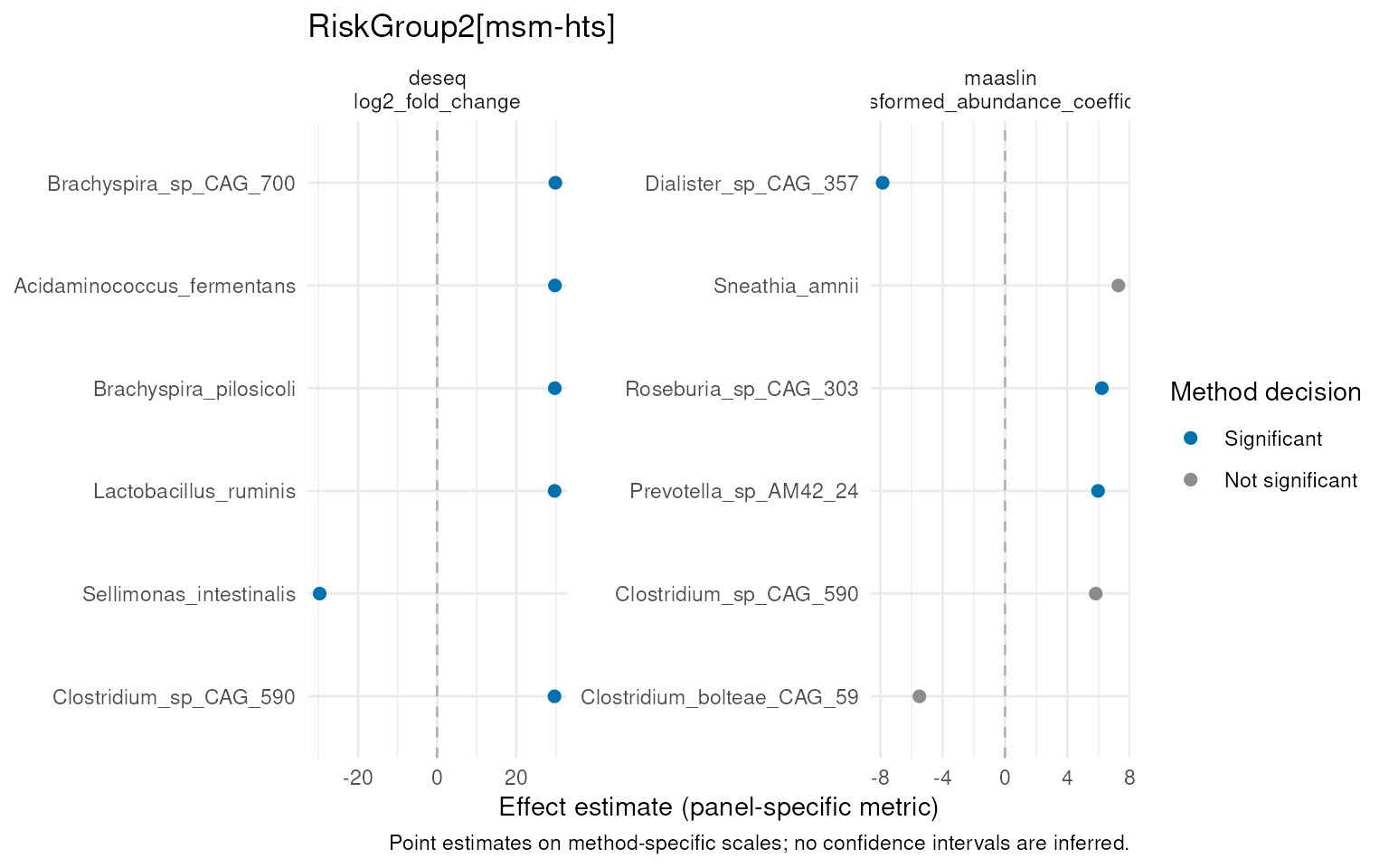
Plots accept explicit contrast selectors so distinct hypotheses are
not mixed. effect_plt() displays each step and effect
metric in a separate panel. Its automatic top_n selects the
largest absolute finite effects within each panel, not the taxa most
supported by other methods. Colours preserve the method’s configured
decision; no universal confidence intervals are inferred.
comparison_id <- "RiskGroup2[msm-hts]"
effect_plt(
  fit, steps = c("deseq", "maaslin"),
  contrast_id = comparison_id, top_n = 6
)
For observed abundances, select discoveries from one configured step
rather than requiring agreement. steps uses the IDs
assigned when the methods were configured. These abundances use the
shared taxonomic analysis view before engine-specific operations; they
are not adjusted model predictions.
abundance_plt(
  fit, steps = "deseq", contrast_id = comparison_id,
  top_n = 6, type = "boxplot"
)
#> You have inserted a phyloseq object. The phyloseq-based methods will be deprecated. We recommend switching to the (Tree)SummarizedExperiment framework and mia R/Bioconductor package.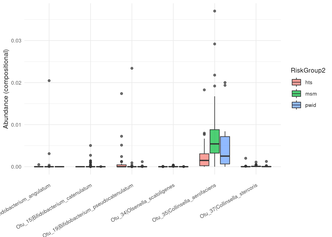
For several steps, choose selection = "union" for
discoveries from any selected step, or selection = "shared"
for those supported by every selected step in the same contrast and
effect direction. An empty selection is valid and does not trigger a
different selection rule. Explicit taxa_ids can also select
taxa independently of significance or agreement.
abundance_plt(
  fit, steps = c("deseq", "maaslin"), selection = "union",
  contrast_id = comparison_id
)
abundance_plt(
  fit, steps = c("deseq", "maaslin"), selection = "shared",
  contrast_id = comparison_id
)
For custom tables and graphics, see tidy_abundance() in
Data inputs and inspection. Optional
agreement plots such as intersection_plt() are described in
their function help. They describe agreement, not statistical accuracy.
bake() defines an optional consensus rule and
cool() extracts its results; their help includes exclusions
and weights. More agreement does not guarantee greater accuracy or
false-discovery rate control, and weights are not probabilities that
methods are correct.
Next steps
- Data inputs and inspection: objects, metadata and units.
- Quality control and preprocessing: QC and filters.
- Statistical models and contrasts: adjustment, repeated measurements and method compatibility.
- Saving and sharing analysis recipes: reusable configurations and the limits of recipe export.
sessionInfo()
#> R version 4.6.1 (2026-06-24)
#> Platform: x86_64-pc-linux-gnu
#> Running under: Ubuntu 24.04.4 LTS
#>
#> Matrix products: default
#> BLAS:   /usr/lib/x86_64-linux-gnu/openblas-pthread/libblas.so.3
#> LAPACK: /usr/lib/x86_64-linux-gnu/openblas-pthread/libopenblasp-r0.3.26.so;  LAPACK version 3.12.0
#>
#> locale:
#>  [1] LC_CTYPE=en_US.UTF-8       LC_NUMERIC=C
#>  [3] LC_TIME=en_US.UTF-8        LC_COLLATE=en_US.UTF-8
#>  [5] LC_MONETARY=en_US.UTF-8    LC_MESSAGES=en_US.UTF-8
#>  [7] LC_PAPER=en_US.UTF-8       LC_NAME=C
#>  [9] LC_ADDRESS=C               LC_TELEPHONE=C
#> [11] LC_MEASUREMENT=en_US.UTF-8 LC_IDENTIFICATION=C
#>
#> time zone: UTC
#> tzcode source: system (glibc)
#>
#> attached base packages:
#> [1] stats     graphics  grDevices utils     datasets  methods   base
#>
#> other attached packages:
#> [1] dar_1.9.12
#>
#> loaded via a namespace (and not attached):
#>   [1] RColorBrewer_1.1-3              jsonlite_2.0.0
#>   [3] MultiAssayExperiment_1.39.1     magrittr_2.0.5
#>   [5] TH.data_1.1-5                   ggbeeswarm_0.7.3
#>   [7] farver_2.1.2                    rmarkdown_2.32
#>   [9] fs_2.1.0                        ragg_1.5.2
#>  [11] vctrs_0.7.3                     multtest_2.69.0
#>  [13] DelayedMatrixStats_1.35.0       SQUAREM_2026.1
#>  [15] mixsqp_0.3-54                   htmltools_0.5.9
#>  [17] S4Arrays_1.13.2                 truncnorm_1.0-9
#>  [19] BiocNeighbors_2.7.3             SparseArray_1.13.4
#>  [21] sass_0.4.10                     bslib_0.12.0
#>  [23] htmlwidgets_1.6.4               desc_1.4.3
#>  [25] sandwich_3.1-3                  plyr_1.8.9
#>  [27] DECIPHER_3.9.3                  zoo_1.9-1
#>  [29] cachem_1.1.0                    igraph_2.3.4
#>  [31] lifecycle_1.0.5                 iterators_1.0.14
#>  [33] pkgconfig_2.0.3                 rsvd_1.0.5
#>  [35] Matrix_1.7-6                    R6_2.6.1
#>  [37] fastmap_1.2.0                   collapse_2.1.8
#>  [39] rbibutils_2.4.1                 MatrixGenerics_1.25.0
#>  [41] numDeriv_2016.8-1.1             digest_0.6.39
#>  [43] S4Vectors_0.51.10               DESeq2_1.53.6
#>  [45] scater_1.41.2                   irlba_2.4.1
#>  [47] textshaping_1.0.5               GenomicRanges_1.65.4
#>  [49] vegan_2.7-6                     beachmat_2.29.3
#>  [51] labeling_0.4.3                  invgamma_1.2
#>  [53] TreeSummarizedExperiment_2.21.0 abind_1.4-8
#>  [55] mgcv_1.9-4                      compiler_4.6.1
#>  [57] withr_3.0.3                     S7_0.2.2
#>  [59] backports_1.5.1                 BiocParallel_1.47.0
#>  [61] viridis_0.6.5                   DBI_1.3.0
#>  [63] MASS_7.3-66                     rappdirs_0.3.4
#>  [65] DelayedArray_0.39.8             biomformat_1.41.0
#>  [67] bluster_1.23.1                  permute_0.9-10
#>  [69] optparse_1.8.2                  tools_4.6.1
#>  [71] vipor_0.4.7                     otel_0.2.0
#>  [73] beeswarm_0.4.0                  ape_5.8-1
#>  [75] glue_1.8.1                      nlme_3.1-171
#>  [77] grid_4.6.1                      Rtsne_0.17
#>  [79] checkmate_2.3.4                 mia_1.21.11
#>  [81] cluster_2.1.8.3                 reshape2_1.4.5
#>  [83] ade4_1.7-24                     generics_0.1.4
#>  [85] microbiome_1.35.1               gtable_0.3.6
#>  [87] tidyr_1.3.2                     data.table_1.18.6.1
#>  [89] utf8_1.2.6                      BiocSingular_1.29.2
#>  [91] ScaledMatrix_1.21.0             XVector_0.53.0
#>  [93] BiocGenerics_0.59.12            ggrepel_0.9.8
#>  [95] foreach_1.5.2                   pillar_1.11.1
#>  [97] stringr_1.6.0                   yulab.utils_0.2.5
#>  [99] emdbook_1.3.14                  splines_4.6.1
#> [101] dplyr_1.2.1                     maaslin3_1.5.7
#> [103] treeio_1.37.1                   lattice_0.23-1
#> [105] survival_3.8-12                 tidyselect_1.2.1
#> [107] DirichletMultinomial_1.55.1     SingleCellExperiment_1.35.2
#> [109] locfit_1.5-9.12                 Biostrings_2.81.9
#> [111] scuttle_1.23.2                  knitr_1.52
#> [113] reformulas_0.4.4                gridExtra_2.3.1
#> [115] phyloseq_1.57.0                 IRanges_2.47.5
#> [117] Seqinfo_1.3.2                   SummarizedExperiment_1.43.0
#> [119] stats4_4.6.1                    xfun_0.61
#> [121] Biobase_2.73.2                  matrixStats_1.5.0
#> [123] stringi_1.8.9                   lazyeval_0.2.3
#> [125] yaml_2.3.12                     evaluate_1.0.5
#> [127] codetools_0.2-20                bbmle_1.0.26
#> [129] tibble_3.3.1                    cli_3.6.6
#> [131] systemfonts_1.3.2               Rdpack_2.6.6
#> [133] jquerylib_0.1.4                 mirai_2.7.3
#> [135] Rcpp_1.1.2                      coda_0.19-4.1
#> [137] nanonext_1.10.3                 bdsmatrix_1.3-7
#> [139] parallel_4.6.1                  pkgdown_2.2.1
#> [141] ggplot2_4.0.3                   sparseMatrixStats_1.25.0
#> [143] mvtnorm_1.4-2                   decontam_1.33.0
#> [145] viridisLite_0.4.3               apeglm_1.35.0
#> [147] tidytree_0.4.8                  scales_1.4.0
#> [149] purrr_1.2.2                     crayon_1.5.3
#> [151] rlang_1.3.0                     multcomp_1.4-32
#> [153] ashr_2.2-63